1.3 How machines learn: neural networks, deep learning and LLMs
1.3 How machines learn: neural networks, deep learning and LLMs
How do machines actually learn? Neural networks form the brain of modern AI – both fascinating and powerful.
Neural networks are modelled on the structure of the human brain: they consist of numerous artificial ‘neurons’ connected to one another via so-called edges. These networks are organised into layers:
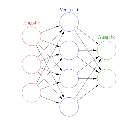 |
Input layer (Eingabe): Receives raw data Hidden layers (Versteckt): Process signals internally Output layer (Ausgabe): Outputs the result In this diagram, there is only one hidden layer. But deep neural networks (Deep Neural Nets) consist of many layers of hidden neurons. Depending on the architecture, the connection patterns of neurons can also vary greatly. |
Architectures: How information flows
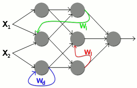 |
In simple networks, information flows only in one direction – from input to output. They are interconnected. These connections are also called edges. Whilst simple neural networks have only forward edges, recurrent networks, for example, also have back edges, through which neurons can influence previous layers. This allows contextual relationships or temporal dependencies to be learnt. |
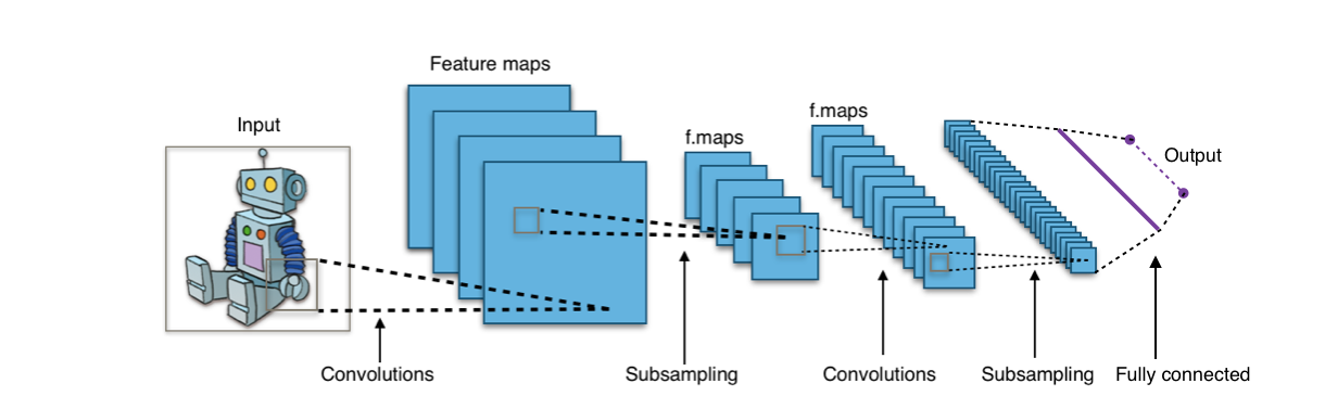
Specialised architectures such as Convolutional Neural Networks (CNNs) are capable of efficiently processing multidimensional inputs such as images or videos.
Information processing: weights and learning
Weights operate between the neurons, determining how strongly a signal is passed on. These weights – also known as parameters – are adjusted during the training of the network. They reflect the knowledge that the model has acquired through learning.
Depending on the weight, the network reacts with varying intensity to specific inputs and thus decides, for example, whether an image is interpreted as a "dog" or a "cat".
How do we arrive at a model that solves a problem?
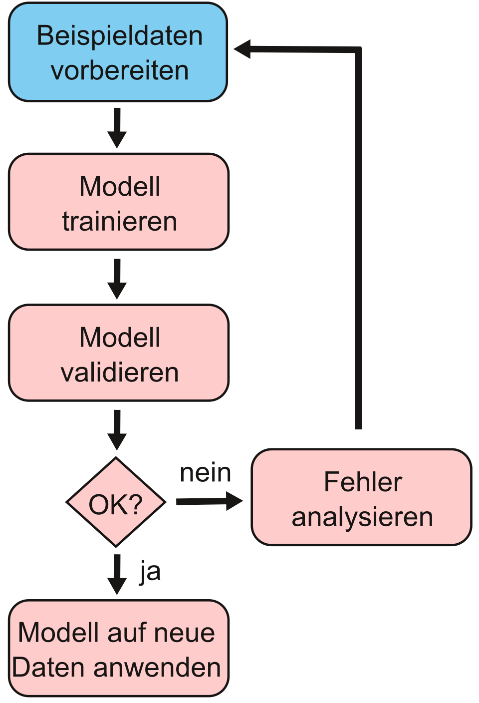 |
A practical example: We want to build a model that distinguishes between images of dogs and cats – a classification problem. To do this, we use a neural network with supervised learning and labelled data (images with unique labels). As neural networks are particularly well-suited to image classification, we use precisely this approach for this problem and have chosen a connectivist approach in line with Domingos’ Five Tribes. To solve a classification problem, we can start from this simplified phase model: Preparation, Training, Testing and Application |
Preparation: Data acquisition and splitting
We collect 2,500 images of dogs and 2,500 images of cats. To label these images, we have various options: we could collect the image filenames in a separate table in one column and note the label "dog" or "cat" in a second column. We could also include the label in each image filename: e.g. Cat1.png, Cat2.png,… Dog1.png,… However, the simplest approach is to save the images of each category in a folder bearing the label name – i.e. all dog images in a "Dog" folder and all cat images in a "Cat" folder.
For the following steps, we divide the images into three groups: we set aside 1,000 images for testing. Of the remaining 4,000 images, we use 3,500 for the actual training and 500 for validation. We’ll come to what that means in a moment. When splitting the data, it is important that we maintain as equal a number of classes as possible (i.e. an equal number of images featuring dogs and cats) in each subset.
How the training works
The training proceeds in stages. In the case of neural networks, we refer to epochs and batches. During each epoch, all 3,500 training images are fed through the neural network once. An epoch is carried out in batches. For each batch, for example, 50 images are fed individually into the network as input and sent forwards through the network, or propagated.
This produces an output value, i.e. a prediction by the current network as to whether the image in question depicts a dog or a cat. This output is compared with the desired result based on the known labels (folder names) of the images.
The difference between the two values is called the error. The average error of the current batch is then used to propagate backwards, i.e. from the output layer back towards the input layer (known as backpropagation). In this process, the weights of the neural connections are adjusted so that the error for these images is reduced in the next step. To determine the precise adjustment of the weights, optimisers such as Stochastic Gradient Descent or the Adam Optimizer are employed.
Through this process, the model gradually learns what a dog or a cat looks like from the colour, brightness and contrast information in the images.
This procedure is repeated for all batches until the network has "seen" all 3,500 training images once.
This is validation
After each epoch, the network’s performance is assessed using the 500 validation images: for example, by measuring accuracy – that is, the number of correctly classified images relative to the total number of images. This allows us to see how accuracy evolves after each epoch and whether the training setup is working overall or not.
If it does not work as desired, so-called hyperparameters can be adjusted: this could be, for example, the architecture of the neural network used, but also the batch size, the number of epochs, or the learning rate, which determines how strongly the weights are adjusted after each batch in accordance with the error during backpropagation.
Training is followed by testing
Finally, the model is tested on the 1,000 test images – to see whether it responds reliably to new data.
Testing on images the model has never seen before is important to check whether we have a model that is also suitable for general use. It is possible that, despite validation, a model may learn the data too precisely or almost ‘by heart’ during training – including errors (overfitting).
Conversely, it is also possible that the model may mistakenly interpret systematic differences in the test images as key distinguishing features. An example would be if dogs in the training images were disproportionately likely to be wearing a collar. The model could then mistakenly conclude that the collar, in particular, indicates that an image depicts a dog.
📌Application example: A model with, for example, 85%+ accuracy can be integrated into a web service for animal image classification.
Model maintenance: When training is not enough
Systematic data issues may have crept in even before the data was split. It could be, for example, that the cat images are systematically brighter than the dog images; in that case, the model might only learn that bright images depict cats and darker images depict dogs. Therefore, monitoring model performance remains relevant even during deployment.
This monitoring is necessary not only to detect such systematic errors, but also to account for changes in the data that users provide for predictions. These changes could arise if new breeds of dogs or cats appear in the application data that were not previously included in the training, validation or test data. This is known as model drift and may require retraining with an updated dataset.
Modern neural networks and how they understand language
The dominant architecture today is the Transformer. It was introduced in 2012 and operates via the so-called self-attention mechanism: this allows the AI, when processing an input (e.g. a sentence), to recognise how strongly each element (e.g. a word) is related to all other elements. The ability to efficiently process contextual relationships across long texts makes Transformers (unlike recurrent neural networks, RNNs) the foundation for models such as Generative Pre-trained Transformers (GPT). This is because they are ideal for language and form the basis for today’s Large Language Models (LLMs) such as ChatGPT, LLaMA or DeepSeek.
LLMs trained on vast amounts of data
LLMs are trained on gigantic amounts of text. Specifically, in the case of the open-source DeepSeek LLM with 67 billion parameters, this amounted to 2 trillion tokens (~word parts, see next section). Assuming that 1 token corresponds to approximately 0.75 words and we have 333 tokens per page (= 250 words), this equates to 6 billion book pages or 10 million books of 600 pages each.
If a token is approximately 4 bytes, this equates to roughly 7.5 terabytes of text data. For DeepSeek’s larger model with 671 billion parameters, as many as 14.8 trillion tokens of training data were used. For Meta’s LLaMA 3.1 models, the figure was 15.6 trillion, and for Alibaba’s Qwen2.5, 18 trillion tokens.
The size of the models and the volume of training data used explain why training requires large data centres with hundreds of GPUs (graphics processing units), yet still takes weeks and is therefore so expensive and energy-intensive.
Why do LLMs understand us at all?
For training LLMs, text is converted into so-called tokens. These are the smallest meaningful units of language, such as words, parts of words, word fragments or punctuation marks. A numerical ID is assigned to these tokens for training.
The example sentence "The cat is sleeping." could be broken down into the following tokens:
["The", "cat", "is", "sleeping", "."]
And these tokens would be assigned corresponding IDs:
["Die" → 101, "Kat" → 202, "ze" → 203, "schläft" → 204, "." → 205],
which would result in the ID sequence
[101, 202, 203, 204, 205]
This can then be fed into the model for training and processing.
Special features of the Transformer architecture and embeddings
The Transformer architecture and the self-attention mechanism are unique because they determine how text is processed further. This takes into account what comes before and after, as well as what the neural network has already learnt. ID tokens are processed differently depending on the context. This means that tokens are converted into embeddings within the model – mathematical vectors with semantic meaning. However, an example illustrates how context is taken into account.
We have these two sentences:
1. "I am sitting on the bank of the river."
2. "I have deposited money into the bank."
We have the word “bank” twice, but with different meanings. This means: Both have the same token ID, but different embeddings – depending on the context. This is how the model recognises different meanings of the same word. Transformer-based LLMs analyse the surrounding words (“of the river” vs. “deposited money”) and generate a specific embedding for each occurrence of “bank” that reflects the respective meaning.
While the first Transformer layers primarily capture local word relationships (e.g. “of the river” vs. “money deposited” for the word “bank”), the representations in the deeper blocks shift increasingly towards global semantics. There, not only word meanings but also grammatical constructions such as co-references are captured. The deeper the layer, the more abstract the relationships: irony, lines of argumentation or the stylistics of a text. This gives rise to thematic and discourse structures that even map dependencies between passages far apart. At these levels, information from the entire context converges, so that when generating responses, the model draws on a deeply integrated, holistic understanding.
The claim that LLMs ‘merely’ predict the next most probable word remains essentially correct, but does not do justice to the complexity of the process.
💡 Learning Summary Chapter 1.3: How machines learn
- Neural networks and deep learning: Artificial neural networks consist of many layers of interconnected units. Their learning performance results from the adjustment of connection weights during training. Deep networks (deep learning) enable particularly powerful applications.
- Transformers and LLMs: Modern LLMs are based on the Transformer architecture with self-attention. They process large amounts of text via so-called tokens, convert these into context-aware embeddings and are capable of flexibly interpreting and generating language.
- Current developments: New methods such as Mixture-of-Experts, Self-Prompting and Chain-of-Thought improve efficiency, problem-solving ability and traceability. Multimodal LLMs additionally integrate image, text and audio processing.
Resources
Transformer: https://arxiv.org/abs/1706.03762
CoT: https://arxiv.org/abs/2201.11903
Tokenisation: https://learn.microsoft.com/de-de/dotnet/ai/conceptual/understanding-tokens
Conversion of identical token IDs into different embeddings depending on context: https://datascience.stackexchange.com/questions/122789/word-embeddings-what-are-contextual-word-embeddings